Operating Systems: Three Easy Pieces 学习笔记(三)
4 The Abstraction: The Process⌗
Process: a running program
4.2 Process API⌗
- create
- destroy
- wait
- miscellaneous control
- status
4.4 Process States⌗
A process can be in one of three states:
- running: executing instructions
- ready: ready to run but the OS has chosen not to run at this moment
- blocked: a process has performed some kind of operation that makes it not ready to run until some other event takes place

5 Interlude: Process API⌗
5.4 Why? Motivating The API⌗
The separation of fork() and exec() is essential in building a UNIX shell, because it lets the shell run code after the call to fork() but before the call to exec(); this code can alter the environment of the about-to-be-run program, and thus enables a variety of interesting features to be readily built.
5.5 Process Control And Users⌗
The user, after entering a password to establish credentials, logs in to gain access to system resources (and as a result, can send signals to programs).
6 Mechanism: Limited Direct Execution⌗
Use time sharing to achieve virtualization
Some challenges:
- performance
- control
6.1 Basic Technique: Limited Direct Execution⌗
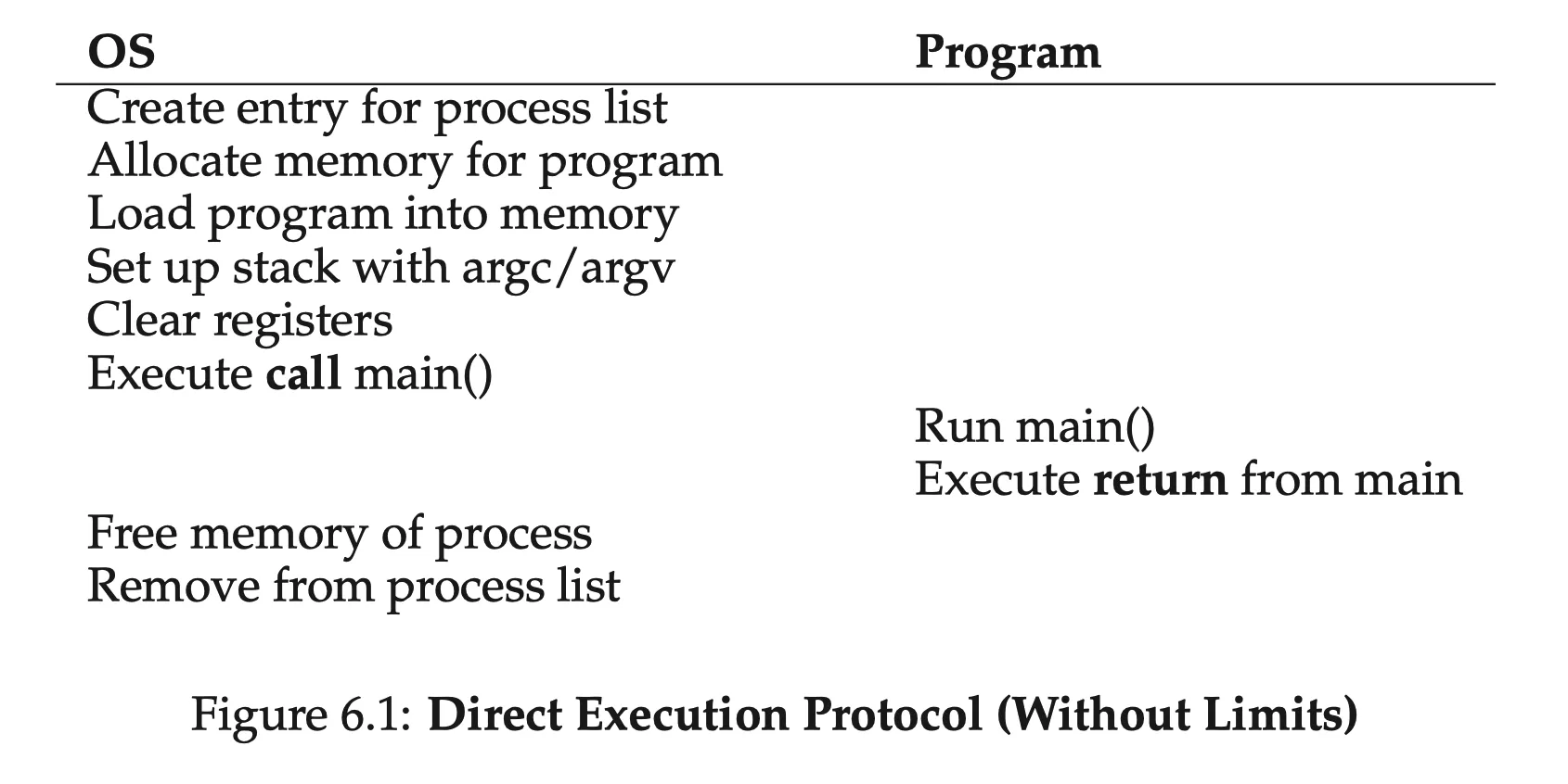
Direct execution: run the program directly on the CPU
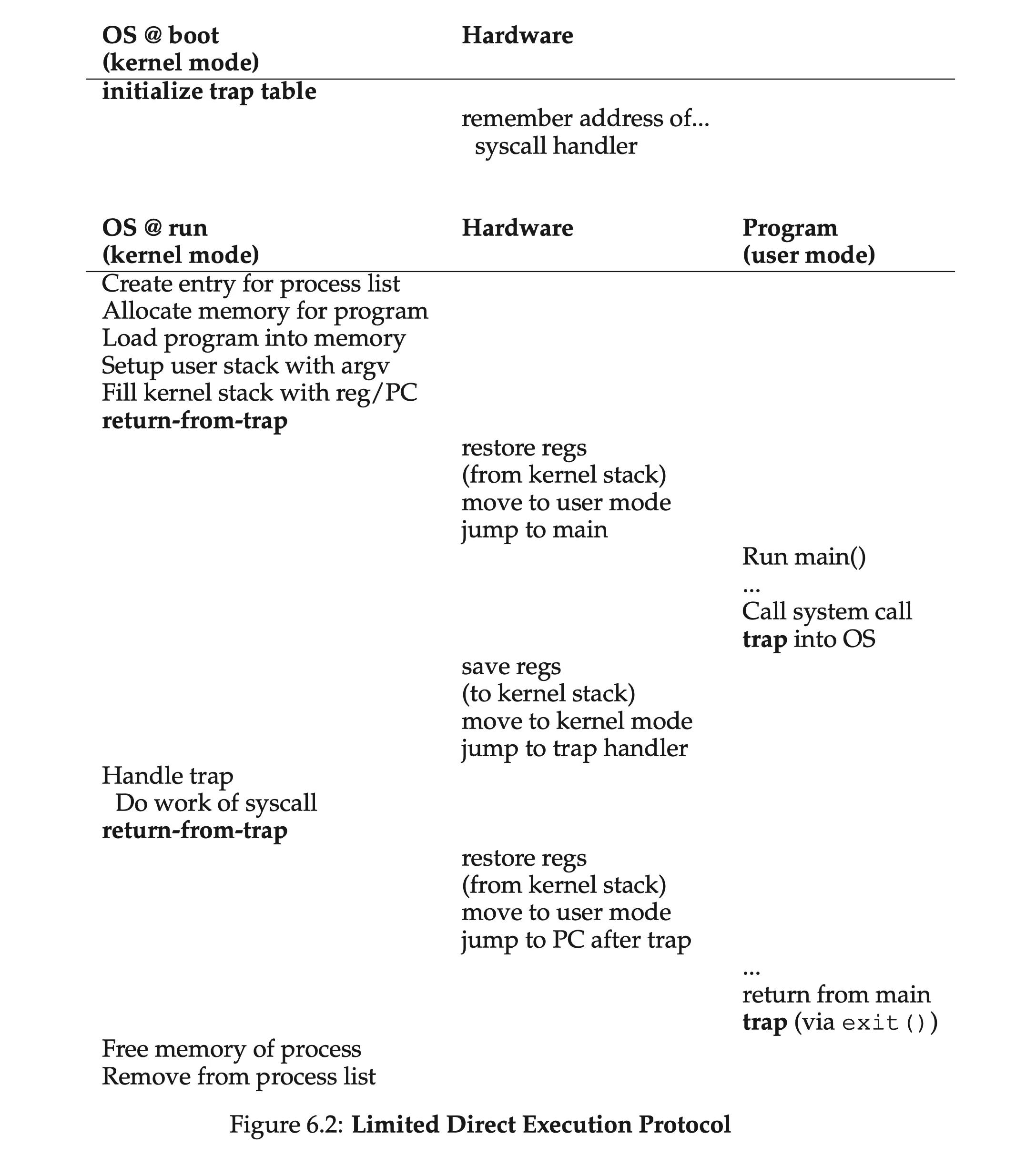
6.2 Problem #1: Restricted Operations⌗
The approach to restrict certain operations: introducing user mode (and kernel mode)
System calls allow the kernel to carefully expose certain key pieces of functionality to user programs, setting up a trap table for the hardware to jump to trap handlers
6.3 Problem #2: Switching Between Processes⌗
The curx: how to regain control of the CPU?
A Cooperative Approach: Wait For System Calls⌗
The OS regains control of the CPU by waiting for a system call or an illegal operation of some kind to take place.
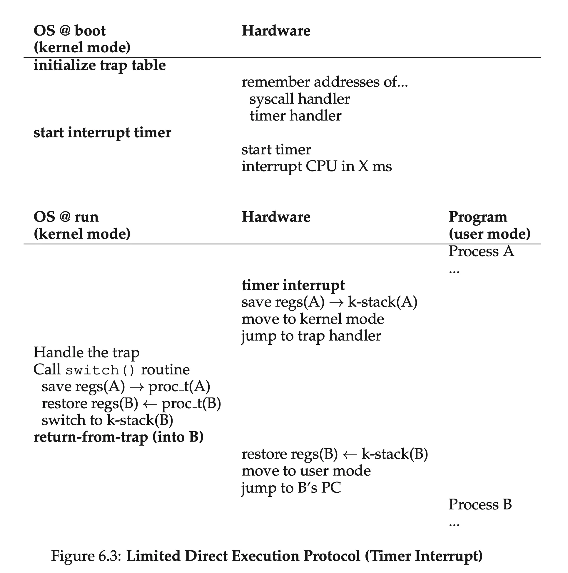
A Non-Cooperative Approach: The OS Takes Control⌗
A timer device can be programmed to raise an interrupt (timer interrupt) every so many milliseconds; when the interrupt is raised, the currently running process is halted, and a pre-configured interrupt handler in the OS runs.
Saving and Restoring Context⌗
Two types of register saves/restores:
- when timer interrupt occurs: the user registers are implicitly saved by the hardware to the kernel stack
- when the OS decides to switch to another process: the kernel registers are explicitly saved by the software to the memory of the process structure (Still in the kernel mode so should kernel registers be saved/restored; the user registers are restored later during return-from-trap)
6.4 Worried About Concurrency?⌗
OS might disable interrupts during interrupt processing (but can lead to lost of interrupts), and use locking to protect concurrent access to internal data structures.
7 Scheduling: Introduction⌗
7.1 Workload Assumptions⌗
Unrealistic assumptions:
- each job runs for the same amount of time
- all jobs arrive at the same time
- once started, each job runs to completion
- all jobs only use the CPU (i.e., they perform no I/O)
- the run-time of each job is known (more unrealistic!)
7.2 Scheduling Metrics⌗
Simplify with one single metric: turnaround time
$$ T_\mathrm{turnaround}=T_\mathrm{completion}-T_\mathrm{arrival} $$
In our case:
$$ T_\mathrm{turnaround}=T_\mathrm{completion} $$
7.3 First In, First Out (FIFO)⌗
The First In, First Out scheduling, or First Come, First Served
Convoy effect: a number of relatively-short potential consumers of a resource get queued behind a heavyweight resource consumer.
7.4 Shortest Job First (SJF)⌗
Shortest Job First: runs the shortest job first, then the next shortest, and so on; optimal.
Bad without assumption 2 (all jobs arrive at the same time)
7.5 Shortest Time-to-Completion First (STCF)⌗
Relax assumption 3 (each job runs to completion)
The scheduler can preempt the current job; adding this to SJF, we get the Shortest Time-to-Completion First (STCF) or Preemptive Shortest Job First (PSJF) scheduler
7.6 A New Metric: Response Time⌗
The response time:
$$ T_\mathrm{response}=T_\mathrm{firstrun}-T_\mathrm{arrival} $$
7.7 Round Robin⌗
Round-Robin: instead of running jobs to completion, RR runs a job for a time slice (sometimes called a scheduling quantum) and then switches to the next job in the run queue
The length of the time slice is critical for RR; a trade-off between response time and the cost of context switching
The cost of context switch
When programs run, they build up a great deal of state in CPU caches, TLBs, branch predictors, and other on-chip hardware. Switching to another job causes this state to be flushed and new state relevant to the currently-running job to be brought in, which may exact a noticeable performance cost.
RR is pretty awful for turnaround time
More generally, any policy (such as RR) that is fair, i.e., that evenly divides the CPU among active processes on a small time scale, will perform poorly on metrics such as turnaround time.
7.8 Incorporating I/O⌗
Relax assumption 4 (all jobs only use the CPU)
Overlap will occur if using STCF
7.9 No More Oracle⌗
Relax our final assumption (the run-time of each job is known)
8 Scheduling: The Multi-Level Feedback Queue⌗
The problem we try to address: given that we in general do not know anything about a process, how to
- optimize turnaround time
- minimize response time
8.1 MLFQ: Basic Rules⌗
The MLFQ has a number of distinct queues, each assigned a different priority level. At any given time, a job that is ready to run is on a single queue.
A job with higher priority (i.e., a job on a higher queue) is chosen to run; use round-robin scheduling among jobs with the same priority.
- rule 1: if Priority(A) > Priority(B), A runs (B doesn’t)
- rule 2: if Priority(A) = Priority(B), A & B run in RR
To set the priority: MLFQ will try to learn about processes as they run, and thus use the history (long-running or interactive) of the job to predict its future behavior.
8.2 Attempt #1: How To Change Priority⌗
- rule 3: when a job enters the system, it is placed at the highest priority
- rule 4
- a: if a job uses up an entire time slice while running, its priority is reduced
- b: if a job gives up the CPU before the time slice is up (therefore jobs with lower priority may have a chance to run), it stays at the same priority level
Example 1: A Single Long-Running Job⌗
Example 2: Along Came A Short Job⌗
The idea: first assumes a job to be short, otherwise move it down; this is an approximization of SJF
Example 3: What About I/O?⌗
Problems With Our Current MLFQ⌗
- starvation: too many interactive jobs will consume all CPU time, thus long-running jobs will never receive any CPU time
- can be attacked by first using most of the time and then perform an I/O
- a program might change its behaviour
8.3 Attempt #2: The Priority Boost⌗
- rule 5: after some time period $S$, move all the jobs in the system to the topmost queue
If $S$ is set too high, long-running jobs could starve; too low, and interactive jobs may not get a proper share of the CPU.
8.4 Attempt #3: Better Accounting⌗
- rule 4: once a job uses up its time allotment (分配) at a given level (regardless of how many times it has given up the CPU), its priority is reduced (i.e., it moves down one queue)
8.5 Tuning MLFQ And Other Issues⌗
9 Scheduling: Proportional Share⌗
The concept: instead of optimizing for turnaround or response time, a scheduler might instead try to guarantee that each job obtain a certain percentage of CPU time.
9.1 Basic Concept: Tickets Represent Your Share⌗
Tickets: the share of a resource that a process (or user or whatever) should receive.
The system picks a ticket (randomly) whose owner process can run at this point
If you are ever in need of a mechanism to represent a proportion of ownership, this concept just might be … (wait for it) … the ticket.
9.2 Ticket Mechanisms⌗
- ticket currency
- ticket transfer
- ticket inflation (通货膨胀)
9.3 Implementation⌗
Best practice: order the list from the highest number of tickets to the lowest
9.4 An Example⌗
Overall fairness is higher with higher job length
9.5 How To Assign Tickets?⌗
Given a set of jobs, the “ticket-assignment problem” remains open.
9.6 Stride Scheduling⌗
Stride: inverse in proportion to the number of tickets a job has
curr = remove_min(queue); // pick client with min pass
schedule(curr); // run for quantum
curr->pass += curr->stride; // update pass using stride
insert(queue, curr); // return curr to queue
Stride scheduling is a deterministic fair-share scheduler.
Lottery scheduling has no global state, so that new processes are easier to be incorporated
9.7 The Linux Completely Fair Scheduler (CFS)⌗
Recent studies have shown that scheduler efficiency is surprisingly important; specifically, in a study of Google datacenters, Kanev et al. show that even after aggressive optimization, scheduling uses about 5% of overall datacenter CPU time.
Basic Operation⌗
Goal: to fairly divide a CPU evenly among all competing processes
In the basic case, each process’s vruntime increases at the same rate, propotional to the physical time. Pick the process with the lowest vruntime to run next.
Divide sched_latency by process number to calculate the time slice; use min_granularity to constrain the minimum possible time slice.
Weighting (Niceness)⌗
Use nice level to control the priority of a process. Positive nice values imply lower priority and negative values imply higher priority
When you’re too nice, you just don’t get as much (scheduling) attention, alas.
Calculation of the time slice:
$$ \texttt{time_slice}_k=\cfrac{\texttt{weight}_k}{\sum_{i=0}^{n-1}\texttt{weight}_i}\cdot\texttt{sched_latency} $$
Also adjusting the calculation of virtual runtime:
$$ \texttt{vruntime}_i=\texttt{vruntime}_i+\cfrac{\texttt{weight}_0}{\texttt{weight}_i}\cdot\texttt{runtime}_i $$
The table preserves CPU proportionality ratios when the difference in nice values is constant
Using Red-Black Trees⌗
Use a red-black tree to maintain running (or runnable) processes; if a process goes to sleep (say, waiting fot an I/O to complete), it is removed.
Dealing With I/O And Sleeping Processes⌗
A just-awaken process will monopolize the CPU; solution: set the vruntime of that job to the min value found in the tree (which only keeps track of running jobs!).
10 Multiprocessor Scheduling (Advanced)⌗
10.1 Background: Multiprocessor Architecture⌗
Two kinds of locality:
- temporal locality
- spatial locality
Problem with multi-code processors: cache coherence; the hardware uses bus snooping to update/invalidate outdated cache
10.2 Don’t Forget Synchronization⌗
10.3 One Final Issue: Cache Affinity⌗
A multiprocessor scheduler should consider cache affinity when making its scheduling decisions, perhaps preferring to keep a process on the same CPU if at all possible.
10.4 Single-Queue Scheduling⌗
Singlequeue multiprocessor scheduling (or SQMS): take an existing policy that picks the best job to run next and adapt it to work on more than one CPU
Problems:
- performance: the overhead of locking is high
- cache affinity: each job ends up bouncing around from CPU to CPU
10.5 Multi-Queue Scheduling⌗
Each CPU has a queue of tasks to be performed.
To solve load imbalance: using migration; a basic approach is to use work stealing